ADMS-Roads

Comprehensive software for modelling road traffic pollution

Model input data

Emissions sources

ADMS-Roads can be used to examine emissions from many sources simultaneously, including:

• Road traffic, over 7000 road links (150 road sources each with up to 50 vertices).
• Industrial sources, up to 3 point, 3 line, 4 area or 25 volume sources.

ADMS-Roads Extra allows for the following sources to be modelled:

• Road traffic, over 25000 road links (600 road sources each with up to 50 vertices).
• Industrial sources, up to 25 point, 5 line, 10 area or 25 volume sources.

Source parameters include:

• source location data,
• road widths and canyon heights for road sources,
• stack heights, diameters, exit velocities, etc., for industrial sources.

Emissions profiles

User-defined emissions profiles can be included in any modelling run to take into account the diurnal variation in traffic flows for individual sources or source groups. Profiles can defined for individual pollutants or for all pollutants from a source.

Seasonal variations can also be included with monthly profiles, or for more detailed modelling, annual hourly profiles can also be modelled.

Emission rates varying with wind direction can also be modelled.

Meteorological data

A variety of meteorological data can be used for input and the format required is deliberately kept very simple.

Wind speed, wind direction and temperature are required along with cloud cover, heat flux or solar radiation.

The meteorological pre-processor calculates the necessary boundary layer parameters from the user's input.

There are a variety of suppliers of meteorological data across the world. A CERC meteorological data converter can convert METAR and other NWS data to ADMS format.

Traffic flow

For road sources, the user can enter hourly speed and traffic flow data into the model and use ADMS-Roads's built-in emission factors to calculate pollutant emission rates, or, alternatively, the user can enter pre-calculated emissions data, for example, emissions calculated within CERC's Emissions Inventory Toolkit, EMIT, which includes many factors such as current and future factors for Euro standard engines.

Modelling roads in urban areas is more complex than just modelling the emissions from traffic as a line source. Both the effect of street canyons and traffic-induced turbulence are included when roads are modelled in ADMS-Roads. Advanced street canyon modelling requires an additional data file containing canyon geometry information for each side of the road.

ADMS-Roads can model the ‘blocking’ effect of elevated road carriageways, which prevent downwards dispersion of emissions within the carriageway. Road tunnels can also be modelled, with emissions automatically moved from the tunnel road to outside the tunnel exit portal and/or a ventilation stack.

Background concentrations

When modelling any local emissions, it is important to include the background concentrations—both ambient concentrations that are advected from outside the modelling area and those that occur due to local emissions that are not explicitly modelled. In the UK, ambient background data can be downloaded from the Defra website (http://uk-air.defra.gov.uk/data/) and included directly in any ADMS-Roads modelling scenario. In ADMS-Roads, background concentrations should be hourly values. If these are not available, constant values can be assumed, but use of an hourly background is preferable.

Model output data[top]

Pollution concentrations can be calculated for averaging times ranging from seconds up to years. ADMS-Roads can calculate percentiles, the number of exceedences of threshold concentrations and rolling averages. These options allow users to compare concentration results directly with appropriate limits, for example those given by the UK NAQS, US NAAQS, EU or WHO.

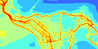
Model results are usually first verified by making comparisons with locally monitored data. This can be done by outputting results at receptor points corresponding to monitoring site locations. Modelled and monitored concentrations can then be compared as a time series plot and the results presented as contour plots. Examples of contour plots showing the impact of a low traffic neighbourhood (LTN) in the London Borough of Lambeth on annual average NO₂ are shown below in the figure below.

<Previous page

Next page>